Many diseases, such as COVID-19, asthma, and other upper respiratory illnesses, are exacerbated by air pollution. Trace gases and particulate matter, for example, aggravate respiratory conditions. Air quality issues are preventable, but prevention requires a knowledge of where vulnerable populations exist and what interventions are needed in those communities. Using observations of trace gases, dust, and other airborne particulate matter combined with socioeconomic data can help do just that.
For more information about aerosol optical depth, trace gas data, and pollutant transport data, please see the Health and Air Quality Data Pathfinder.
Image

AOD is a column-integrated value of aerosols in the atmosphere obtained by measuring the scattering and absorption of solar energy from the top of the atmosphere to the surface. The non-aerosol signal of surface reflectance needs to be separated from the aerosol signal to accurately obtain an AOD. This is challenging because the satellite instrument cannot penetrate cloud cover and highly reflective surfaces, such as ice or snow. This, in turn, can lead to misrepresentations in the data. To address this, scientists developed algorithms for data acquired by the Moderate Resolution Imaging Spectroradiometer (MODIS): the Dark Target algorithm and the Deep Blue algorithm. In the latest MODIS dataset collection, these two algorithms have been merged, using the highest quality for each.
The Visible Infrared Imaging Radiometer Suite (VIIRS), aboard the joint NASA/NOAA Suomi National Polar-orbiting Partnership (Suomi NPP) satellite, also collects AOD data, but at a finer spatial resolution. VIIRS uses the Deep Blue algorithm over land and the Satellite Ocean Aerosol Retrieval (SOAR) algorithm over water to determine atmospheric aerosol loading for daytime cloud-free, snow-free scenes. Downloading a VIIRS data file will provide data with just the land algorithm, just the ocean algorithm, and the merged algorithm. As with all remote sensing data, make sure you are choosing the best product for your area and use.
Data Products for Measuring AOD
Research quality data products can be accessed using Earthdata Search (data are in HDF or NetCDF format, and can be opened using NASA'S Panoply application):
- MODIS/Aqua AOD (3km resolution, merged algorithm)
- MODIS/Terra AOD (3km resolution, merged algorithm)
- MODIS Terra/Aqua-MAIAC Retrieval AOD
Multi-angle Implementation of Atmospheric Correction (MAIAC) Land AOD utilizes a new advanced algorithm which uses time series (TMS) analysis and a combination of pixel- and image-based processing to improve the accuracy of cloud detection, aerosol retrievals, and atmospheric correction. - VIIRS AOD at 1 degree x 1 degree (daily global data coverage)
- VIIRS AOD at 6 km (daily)
- Monthly VIIRS AOD at 1 degree x 1 degree
Data products can be visualized as a time-averaged map, an animation, seasonal maps, scatter plots, or a time series through an online interactive NASA data analysis tool called Giovanni. Follow these steps to plot data in Giovanni: 1) Select a map plot type; for more information on choosing a type of plot, see the Giovanni User Manual. 2) Select a date range. Data are in multiple temporal resolutions, so be sure to note the start and end date to ensure you access the desired dataset. 3) Check the box of the variable in the left column that you'd like to include and then plot the data.
- OMI AOD in Giovanni
The Ozone Monitoring Instrument (OMI) aboard the Aura satellite has a coarser spatial resolution than MODIS and VIIRS, but provides data at individual wavelengths from the ultraviolet (UV) to the visible. Within Giovanni, you can plot daily data at these individual wavelengths. This is important because pollutants have different spectral signatures; for example, a wavelength range around 400 nm can be used to detect elevated layers of absorbing aerosols such as biomass burning and desert dust plumes. The two AOD products provided through Giovanni use two different algorithms: OMI Multi-wavelength (OMAERO) and OMI UV (OMAERUV). OMAERO is based on the multi-wavelength algorithm and uses up to 20 wavelength bands between 331 nm and 500 nm. This algorithm uses reflectance for a wide variety of microphysical aerosol models representative of desert dust, biomass burning, volcanic, and weakly absorbing aerosol types. OMAERUV uses the near-UV algorithm, which is capable of retrieving aerosol properties over a wider variety of land surfaces than is possible using measurements only in the visible or near-IR. - MODIS AOD in Giovanni
Provides data products with both the Dark Target and Deep Blue algorithms, as well as the combined Dark Target/Deep Blue algorithm at daily and monthly intervals.
Near real-time data, which are available generally within three hours of a satellite observation through LANCE, can be visualized and interactively explored using NASA Worldview:
- MODIS Aqua/Terra Combined Algorithm AOD
The merged Dark Target/Deep Blue AOD layer provides a more global, synoptic view of AOD over land and ocean. It is available from 2000 to present. - VIIRS Level 2 Deep Blue Aerosol Product
The product uses the Deep Blue algorithm over land and the SOAR algorithm over water to determine atmospheric aerosol loading. The product is designed to facilitate continuity in the aerosol record. Deep Blue uses measurements from multiple Earth observing satellites to determine the concentration of atmospheric aerosols along with the properties of these aerosols. - OMI AOD Multi-wavelength and UV
The multi-wavelength layer and the UV absorbing layer displays the degree to which airborne particles (aerosols) prevent the transmission of light through the process of absorption (attenuation). The UV extinction layer indicates the level at which aerosols prevent light from traveling through the atmosphere. Toggling between these layers can help distinguish the types of aerosols present.
Image

As mentioned above, AOD is the quantity of light removed from a beam by scattering or absorbing during its path through a medium and is a unitless measure. PM2.5, on the other hand, is a measure of the mass of particles in a specific size range (generally 2.5 micrometers and smaller) within a given volume of air near the surface. Particles less than 10 micrometers in diameter pose a significant health threat because they can get deep into lungs, and some may even get into the bloodstream, according to the U.S. EPA). There are a few differences between AOD and PM2.5:
- AOD is an optical measurement; PM2.5 is a mass concentration measurement.
- AOD is an integrated column measurement from the top of the atmosphere to the surface; PM2.5 is a ground measurement.
- AOD is an area-averaged measurement; PM2.5 is a point measurement.
Because the two measurements are so different, it may seem that there is no correlation. However, they do correlate and there are several techniques to convert AOD to PM2.5. It is important to note that while there is a relationship between AOD and PM2.5, there are other factors that can affect AOD, like humidity, the vertical distribution of aerosols, and the shape of the particles. For example, an increase in humidity will increase the size of particles and therefore increase the AOD even though the PM2.5 level will be the same.
Ground-based AOD measurements are available online through the Aerosol Robotic Network (AERONET). The EPA's ground-based PM and Ozone combined Air Quality Index (AQI) can be accessed at AirNow.
NASA's Applied Remote Sensing Training (ARSET) program has a Jupyter Notebook available through the ARSET GitHub site that accesses VIIRS AOD data and converts AOD to PM2.5. For more information on using this notebook, view the ARSET MODIS to VIIRS Transition for Air Quality Applications.
For trends in PM2.5, there are several resources that utilize both ground-based and remote sensing data:
- PM <2.5 micrometers in Worldview (data are available from 2001-2012)
- Worldbank global mean exposure to PM2.5
Nitrogen Dioxide (NO2) is a pollutant that can aggravate respiratory conditions in humans, especially those with asthma, leading to an increase of symptoms, hospital admissions, and emergency visits. The primary sources of NO2 are fossil fuel burning, automobile exhaust, and industry emissions. Long-term exposure can lead to the development of asthma and potentially increase susceptibility to respiratory infections. NO2 reacts with other chemicals in the atmosphere, forming particulate matter and ozone, producing haze and acid rain, and contributing to nitrogen pollution in coastal waters. The NASA Air Quality site provides more information on NO2, as well as trend maps and pre-made images of NO2 over cities and power plants.
Image

Research quality data products can be accessed using Earthdata Search:
- OMI NO2 data
The OMI sensor aboard the Aura spacecraft provides daily gridded and non-gridded products at 13x24 km resolution; data are in HDF5 format, and can be opened using NASA's Panoply application. A tutorial on using OMI NO2 data is available as a PDF and a webinar on Analyzing NO2 data within Java and Excel is available from the Earthdata YouTube website. - TROPOMI NO2 data
The TROPOspheric Monitoring Instrument (TROPOMI) is aboard the European Space Agency (ESA) Sentinel-5 satellite. ESA's TROPOMI NO2 data website provides additional information on this Level 2 data product. Data are in NetCDF format, and can be opened using Panoply. Because of the very small values in tropospheric vertical column of NO2, you will need to change the scaling factor in Panoply (see image from June 2018 at right).
Data products can be visualized as a time-averaged map, an animation, seasonal maps, scatter plots, or a time series through an online interactive NASA data analysis tool called Giovanni. Follow these steps to plot data in Giovanni: 1) Select a map plot type; for more information on choosing a type of plot, see the Giovanni User Manual. 2) Select a date range. Data are in multiple temporal resolutions, so be sure to note the start and end date to ensure you access the desired dataset. 3) Check the box of the variable in the left column that you'd like to include and then plot the data.
Near real-time data can be visualized and interactively explored using NASA Worldview:
- OMI NO2
- Trends over time: Ground level NO2 (data are from 1996-1998 and 2010-2012)
NASA also has a global nitrogen dioxide monitoring site that provides imagery of daily NO2 from OMI.
The Aerosol Index (AI) is a measurement related to AOD and indicates the presence of an increased amount of suspended particles in the atmosphere. High concentrations of aerosols can exacerbate conditions like asthma, bronchitis, and other respiratory conditions. The main aerosol types included in the AI are desert dust, large fire events, biomass burning, and volcanic ash plumes. The lower the AI, the clearer the sky.
Image

Research quality data products can be accessed using Earthdata Search:
- OMI AI
OMI provides an Ultraviolet Aerosol Index; data are in HDF5 format, and can be opened using NASA's Panoply application. Note that when opening the data in Panoply, there are a number of different data fields from which to choose. Select UVAerosolIndex. - TROPOMI AI data
ESA TROPOMI AI provides additional information on this Level 2 data product. Data are in NetCDF format, and can be opened using Panoply.
Data products can be visualized as a time-averaged map, an animation, seasonal maps, scatter plots, or a time series through an online interactive NASA data analysis tool called Giovanni. Follow these steps to plot data in Giovanni: 1) Select a map plot type; for more information on choosing a type of plot, see the Giovanni User Manual. 2) Select a date range. Data are in multiple temporal resolutions, so be sure to note the start and end date to ensure you access the desired dataset. 3) Check the box of the variable in the left column that you'd like to include and then plot the data.
Near real-time data can be visualized and interactively explored using NASA Worldview:
- OMI AI data
- OMPS AI data
OMPS AI layer indicates the presence of ultraviolet (UV)-absorbing particles in the air.
Image

The Dust Score indicates the level of atmospheric aerosols. The numerical scale is a qualitative representation of the presence of dust in the atmosphere, an indication of where large dust storms may form, and the areas that may be affected. Near real-time data can be visualized and interactively explored using NASA Worldview:
- AIRS Dust Score
Measurement from the Atmospheric Infrared Sounder (AIRS) Infrared quality assurance subset; the imagery resolution is 2 km.
Image
")
Many diseases, such as Rift Valley fever, cholera, chikungunya, and dengue are generally found in tropical regions with poor water quality and sanitation coupled with limited access to health care services. For example, cholera is contracted from consuming water or food contaminated with the the toxic bacterium Vibrio cholerae. According to the Centers for Disease Control and Prevention (CDC), an estimated 2.9 million cases of cholera and 95,000 deaths from the disease occur each year around the world.
Cholera occurs in two forms: endemic and epidemic. The endemic form of cholera occurs during the dry season, when freshwater river levels are low and saltwater can more easily penetrate into coastal areas. The extra salt provides a good habitat for the growth of algae, which draws in small crustaceans called copepods that feed on the floating vegetation and are a vector for cholera. This brings copepods closer to sources of water used for drinking, sanitation, and bathing. The epidemic form of cholera, in contrast, occurs suddenly and sporadically. These outbreaks typically occur after a disaster such as when flooding contaminates clean water sources or damages water infrastructure.
The Water Quality Data Pathfinder has additional information on the integration of ground-based data with satellite or airborne data for assessing water quality.
Image

In addition to ocean color, sea surface temperature (SST) is a valuable parameter in evaluating the growth of algal blooms. Depending on the species of cyanobacteria involved, toxins in these blooms can affect the central nervous system (neurotoxins), the liver (hepatotoxins), and other systems.
The inherent optical properties (IOP) file in MODIS and VIIRS data provides an estimate of reflectance by CDOM. Specifically, the adg_443_giop is the absorption coefficient of non-algal material plus CDOM. For more information on the algorithm used to generate this product and others, see Algorithm Descriptions at NASA's Ocean Biology DAAC (OB.DAAC).
Research-quality data products can be accessed through NASA partner websites, Earthdata Search, or OB.DAAC:
- Landsat Data from USGS Earth Explorer
Landsat is a joint NASA/USGS program that provides the longest continuous space-based record of Earth's land. On the Earth Explorer site, specify your search criteria then:- Select "Data Sets"
- Select Landsat
- Select Landsat Collection 1 Level-1
- Select Landsat 7 and/or Landsat 8
- MODIS Ocean Color/IOP level 2 data from Earthdata Search
Terra/MODIS SST level 2 data from Earthdata Search
These datasets are available in NetCDF format, and can be opened using SeaDAS or other NASA-developed tools. - VIIRS Ocean Color level 2 data from Earthdata Search
VIIRS IOP level 2 data from Earthdata Search
VIIRS SST level 2 data from Earthdata Search
These datasets are available in NetCDF format, and can be opened with SeaDAS or other NASA-developed tools. - Sentinel-3 OLCI data from Earthdata Search
Data are available in NetCDF format within zip files. - Level 1 and 2 data from OB.DAAC
Algorithms are available through the SeaDAS program to derive ocean color products from this Level 1 and 2 data, if needed. - Level 3 data from OB.DAAC
Data products include chlorophyll-a concentration, sea surface temperature (SST), reflectance, and other related measurements from MODIS and VIIRS at 4 km and 9 km resolution. These data products are provided in five temporal resolutions: daily, 8-day, monthly, seasonally, and annually.
Data products can be visualized as a time-averaged map, an animation, seasonal maps, scatter plots, or a time series through an online interactive NASA data analysis tool called Giovanni. Follow these steps to plot data in Giovanni: 1) Select a map plot type; for more information on choosing a type of plot, see the Giovanni User Manual. 2) Select a date range. Data are in multiple temporal resolutions, so be sure to note the start and end date to ensure you access the desired dataset. 3) Check the box of the variable in the left column that you'd like to include and then plot the data.
- Data products from MODIS on the Aqua satellite at 4 km resolution provided at both 8-day and monthly temporal resolutions:
Near real-time data can be visualized and interactively explored using NASA Worldview:
Image

Salinity, the amount of salt dissolved in seawater, drives ocean currents that transport heat around the globe. Drinking water with high saline concentrations has been identified as an increasing public health concern due to its contributions to cardiovascular and other diseases. Two missions have been measuring SSS since 2011: the international Aquarius/Satélite de Aplicaciones Científicas (SAC)-D observatory, which carries NASA's Aquarius instrument, and NASA's Soil Moisture Active Passive (SMAP) satellite.
Aquarius Version 5 is the official end-of-mission dataset, spanning the complete period of Aquarius science data availability from August 2011 to June 2015. Improving the accuracy of Aquarius' measurements has been a key mission activity to ensure that the data are most useful for science and society. There are two products: the official release and another from NASA's Jet Propulsion Laboratory (JPL) based on the Combined Active Passive (CAP) retrieval algorithm.
While SMAP is designed to measure soil moisture over land, algorithm development from the Aquarius mission is applied to SMAP data to derive SSS. There are two SMAP SSS products, one from JPL and one from a private company called Remote Sensing Systems (RSS). The JPL product is based on the CAP retrieval algorithm and provides a comparative view to RSS, which is based on averages spanning an 8-day moving window.
Note that the Aquarius data are only available from 2011–2015 and are at a much coarser spatial resolution than SMAP. The SMAP data record begins in March/April 2015.
Research-quality SSS data products can be accessed using Earthdata Search:
For subsetting SSS data, use the HiTIDE Tool available through NASA's Physical Oceanography DAAC (PO.DAAC) (see the Tools for Data Access and Visualization section for more information)
SSS data can be visualized using Worldview and PO.DAAC's State of the Ocean (SOTO) tool:
- Aquarius SSS data in Worldview
- SMAP SSS data in Worldview
- Aquarius SSS data in SOTO
- SMAP SSS data in SOTO
Image
 field-based campaigns.")
Field-based campaigns provide SSS data on a regional level. Salinity Processes in the Upper Ocean Regional Study (SPURS) is a pair of oceanographic field experiments using a variety of equipment and technology, including salinity-sensing satellites, research cruises, floats, drifters, autonomous gliders, and moorings. The 2012–2013 SPURS-1 field campaign in the North Atlantic focused on a high salinity, high evaporation region. The 2016–2017 SPURS-2 field campaign is the center of the low surface salinity belt associated with the heavy rainfall of the intertropical convergence zone in the Tropical Pacific.
Saildrone is a state-of-the-art, wind-and-solar-powered Uninhabited Surface Vehicle (USV) capable of long distance deployments lasting up to 12 months. This novel sampling platform is equipped with a suite of instruments and sensors providing high quality, georeferenced, near real-time, multi-parameter surface ocean and atmospheric observations.
Research-quality field-based salinity data can be accessed using Earthdata Search:
Image
 in Central and Eastern Canada from 2000 to 2015, with red indicating a high risk of encountering this tick species. Image from Kotchi, S.O., et al., 2021 (doi:10.3390/rs13030524).")
Vector-borne diseases are human illnesses caused by viruses and bacteria transmitted from mosquitoes, fleas, ticks, and similar sources. According to the WHO, diseases such as dengue, malaria, chikungunya, yellow fever, and Zika cause more than 700,000 deaths per year and disproportionately affect the poorest populations in tropical regions. Lyme disease is one of the primary vector-borne diseases in the temperate region of the North Hemisphere. The distribution of vector-borne diseases is determined by a complex set of demographic, environmental, and social factors. Also, the expansion of these diseases into other areas is accelerating as the global climate warms and habitats change. For more details on vector-borne diseases, please see Of Mosquitoes and Models: Tracking Disease by Satellite.
Scientists can predict vector distributions by identifying key environmental characteristics of suitable species habitats, such as areas of standing water that are breeding grounds for mosquito larvae. Measurements from NASA, including land use/land cover, precipitation, temperature, and vegetation indices, can help identify potentially suitable vector habitats.
Image

Land cover type can provide information about potential larval habitats. Different mosquito species are often associated with different land cover characteristics. In the Amhara region of Ethiopia, for example, lowland pastures are important breeding sites for anopheline mosquitoes; as a result, landscapes with a high proportion of these wetlands have higher incidences of malaria.
The Terra and Aqua MODIS Land Cover Type data product provides global land cover types at yearly intervals that are derived from six different classification schemes (the MODIS Land Cover User Guide provides additional information on these schemes). The product is derived using supervised classifications of MODIS Terra and Aqua reflectance data. The supervised classifications then undergo additional post-processing that incorporate prior knowledge and ancillary information to further refine specific classes.
Image

Land surface temperature is useful for monitoring changes in weather and climate patterns that can impact the suitability of an area for a specific species to live and function. For example, there are different optimum temperature ranges for the transmission of different mosquito-borne diseases in various ecological contexts.
Research quality land surface temperature data products can be accessed directly from Earthdata Search (these data also are available through NASA's Land Processes DAAC [LP DAAC] Data Pool). MODIS and ASTER data are available in HDF format while data from VIIRS and the ECOsystem Spaceborne Thermal Radiometer Experiment on Space Station (ECOSTRESS) are available in HDF5 format:
- Terra MODIS Land Surface Temperature
- Aqua MODIS Land Surface Temperature
For both of the MODIS products, select daily, 8-day, or monthly at 1 km or 5.6 km resolution. For more information on spatial and temporal resolution, see What is Remote Sensing? - Terra MODIS Land Surface Temperature/3-Band Emissivity
- Aqua MODIS Land Surface Temperature/3-Band Emissivity
For both of these MODIS products, select 5-min, daily, and 8-day at 1 km resolution. - VIIRS Land Surface Temperature
- VIIRS Land Surface Temperature/3-Band Emissivity
Choose daily or 8-day at 1 km resolution. - ASTER Surface Kinetic Temperature
ASTER Surface Temperature products are processed on-demand and so must be requested with additional parameters. Note that there is a limit to 2,000 granules per order. - ECOSTRESS Land Surface Temperature
To quickly extract a subset of ECOSTRESS, MODIS, or VIIRS data for your region of interest, use LP DAAC's Application for Extracting and Exploring Analysis Ready Samples (AppEEARS) tool or NASA's Oak Ridge National Laboratory DAAC's (ORNL DAAC) subsetting tools.
Landsat data can be discovered using Earthdata Search (you will need a USGS Earth Explorer login to download Landsat data):
- Landsat 8 Thermal Infrared Sensor
Measures land surface temperature in two thermal bands with a new technology that utilizes quantum physics to detect heat.
Data can be visualized and interactively explored using Worldview:
The NASA Earth Exchange Global Daily Downscaled Projections Coupled Model Intercomparison Project Phase 6 (NEX-GDDP-CMIP6) dataset is comprised of high-resolution, bias-corrected global downscaled climate projections derived from the General Circulation Model (GCM) runs conducted under the Coupled Model Intercomparison Project Phase 6 (CMIP6) and across all four “Tier 1” greenhouse gas emissions scenarios known as Shared Socioeconomic Pathways (SSPs).
This dataset provides a set of global, high resolution, bias-corrected climate change projections that can be used to evaluate climate change impacts on processes that are sensitive to finer-scale climate gradients and the effects of local topography on climate conditions. Uses include: air temperature, precipitation volume, humidity, stellar radiation, and atmospheric wind speed.
NEX-GDDP-CMIP6 data are available through the NASA Center for Climate Simulation (NCCS):
Image

Vegetation indices are a proxy measure of green vegetation over a given area and can be used to assess vegetation health. Vegetation indices, in particular the Normalized Difference Vegetation Index (NDVI), can be used to describe habitat suitability for different species of disease-carrying vectors, such as mosquitoes. NDVI uses the difference between near-infrared (NIR) and red reflectance divided by their sum. NDVI values range from -1 to 1. Low values of NDVI generally correspond to barren areas of rock, sand, exposed soils, or snow; higher NDVI values indicate greener vegetation, including forests, croplands, and wetlands. The enhanced vegetation index (EVI) is another widely used vegetation index that minimizes canopy-soil variations and improves sensitivity over areas of dense vegetation.
Vegetation products produced from data acquired by MODIS and VIIRS can be accessed in various ways.
Research-quality data products can be accessed directly using Earthdata Search (these data also are available through the LP DAAC Data Pool). Datasets are available in HDF format (in some cases they are customizable to GeoTIFF):
LP DAAC's AppEEARS offers a simple and effective way to extract, transform, visualize, and download MODIS and VIIRS vegetation-related data products. AppEEARS allows users to subset data by defining specific point(s) or area(s) of interest, and output data can be downloaded in csv (point), GeoTIFF (area), or NetCDF4 (area) format. Explore LP DAAC's Getting Started with Cloud-Native Harmonized Landsat Sentinel (HLS) Data in Python Jupyter Notebook for extracting an EVI Time Series from HLS. ORNL DAAC subsetting tools provide a means to simply and efficiently access and visualize MODIS and VIIRS vegetation-related data products, as well.
Data products can be visualized as a time-averaged map, an animation, seasonal maps, scatter plots, or a time series through an online interactive NASA data analysis tool called Giovanni. Follow these steps to plot data in Giovanni: 1) Select a map plot type; for more information on choosing a type of plot, see the Giovanni User Manual. 2) Select a date range. Data are in multiple temporal resolutions, so be sure to note the start and end date to ensure you access the desired dataset. 3) Check the box of the variable in the left column that you'd like to include and then plot the data.
- MODIS NDVI in Giovanni
Data can be downloaded in GeoTIFF format.
Vegetation indices can be visualized and interactively explored in Worldview:
- MODIS NDVI
This dataset has a spatial resolution of 250 m and a temporal resolution of eight days. 16-day and monthly data are also available through Worldview. - MODIS EVI
This dataset is monthly at 1 km spatial resolution. Rolling 8-day and 16-day data are also available through Worldview.
Image

Precipitation is the ultimate source of water for the aquatic habitats of mosquito larvae. However, the direct effects of precipitation on larval survival are highly varied and are not always positive. For example, heavy rain can cause flooding, which can result in high levels of larval mortality. In addition, the effects of rainfall on breeding habitats are highly contingent upon local conditions, such as soil saturation, topography, and land use.
NASA's Precipitation Measurement Missions (PMM) provide a continuous long-term record (over 20 years) of precipitation data through the Tropical Rainfall Measuring Mission (TRMM) and the Global Precipitation Measurement (GPM) mission. GPM, a TRMM follow-on mission, provides more accurate measurements, improved detection of light rain and snow, and extended spatial coverage.
TRMM and GPM products are available individually and have been integrated with data from a global constellation of satellites to yield improved spatial/temporal precipitation estimates providing a temporal resolution of 30 minutes (in the case of GPM). The integrated products are the TRMM Multi-satellitE Precipitation Analysis (TMPA) and the Integrated Multi-satellite Retrievals for GPM (IMERG). IMERG's multiple runs accommodate different user requirements for latency and accuracy (Early = 4 hours, e.g., for flash flood events; Late = 12 hours, e.g., for crop forecasting; and Final = 3 months, with the incorporation of rain gauge data, for research).
NASA, in collaboration with other agencies, has developed precipitation models that incorporate satellite information with ground-based data. These models are part of the Land Data Assimilation System (LDAS), which includes a global collection (GLDAS) and a North American collection (NLDAS). LDAS uses inputs including precipitation, soil texture, topography, and leaf area index to create model output estimates.
Science quality data products can be accessed using Earthdata Search:
- TMPA
Rainfall estimate at 3 hours, 1 day, or NRT and accumulated rainfall at 3 hours and 1 day. Data are in HDF format and can be opened using NASA's Panoply application. Data are available from 1997. - IMERG
Early, Late, and Final precipitation data on the half hour or 1-day timeframe. Data are in NetCDF or HDF format, and can be opened using Panoply. Data are available from 2000.
Data products can be visualized as a time-averaged map, an animation, seasonal maps, scatter plots, or a time series through an online interactive NASA data analysis tool called Giovanni. Follow these steps to plot data in Giovanni: 1) Select a map plot type; for more information on choosing a type of plot, see the Giovanni User Manual. 2) Select a date range. Data are in multiple temporal resolutions, so be sure to note the start and end date to ensure you access the desired dataset. 3) Check the box of the variable in the left column that you'd like to include and then plot the data.
Near real-time data can be accessed using Worldview:
- IMERG Precipitation Rate
- AMSR2 Precipitation Rate
The Advanced Microwave Scanning Radiometer 2 (AMSR2) instrument collects data that indicate the rate at which precipitation is falling on the ocean surface and is measured in millimeters per hour (mm/hr). - NLDAS Precipitation Total
- GLDAS Precipitation Total (only goes through 2010)
The NLDAS monthly Precipitation Total data are generated through temporal accumulation of the hourly data, and the GLDAS monthly data are generated through temporal averaging of the 3-hourly data. The data are in kg/m2/s which is equivalent to mm/s.
In addition, the IMERG Early Run Half-Hourly product is available through NASA's PMM website. This product is generated every half hour with a 6-hour latency from the time of data acquisition
Daymet is a collection of gridded estimates of daily weather parameters, and is available through ORNL DAAC. It is modeled on daily meteorological observations. Weather parameters in Daymet include daily minimum and maximum temperature, precipitation, vapor pressure, radiation, snow water equivalent, and day length at 1 km resolution over North America, Puerto Rico, and Hawaii.
Daymet data can be retrieved using Earthdata Search, an ORNL DAAC API, ORNL DAAC tools, and through LP DAAC AppEEARS.
The NASA Earth Exchange Global Daily Downscaled Projections Coupled Model Intercomparison Project Phase 6 (NEX-GDDP-CMIP6) dataset is comprised of high-resolution, bias-corrected global downscaled climate projections derived from the General Circulation Model (GCM) runs conducted under the Coupled Model Intercomparison Project Phase 6 (CMIP6) and across all four “Tier 1” greenhouse gas emissions scenarios known as Shared Socioeconomic Pathways (SSPs).
This dataset provides a set of global, high resolution, bias-corrected climate change projections that can be used to evaluate climate change impacts on processes that are sensitive to finer-scale climate gradients and the effects of local topography on climate conditions. Uses include: air temperature, precipitation volume, humidity, stellar radiation, and atmospheric wind speed.
NEX-GDDP-CMIP6 data are available through the NASA Center for Climate Simulation (NCCS):
Image

For diseases transmitted by vectors without an aquatic development stage, such as ticks and sandflies, relative humidity exerts a strong influence on vector survival. In general, both very low and very high temperatures increase tick mortality rates; however, an increase in humidity can increase the ability of ticks to tolerate higher temperatures. In addition, temperature coupled with humidity can also influence the timing of host-seeking activity and can influence the seasons of highest risk to the public, according to the U.S. Global Change Research Program.
Research-quality data products can be accessed using Earthdata Search:
- AIRS Relative Humidity
Data from AIRS are available daily at 1 degree, and Level 3 data products are provided in either the descending (equatorial crossing north to south at 1:30 a.m. local time) or ascending (equatorial crossing south to north at 1:30 p.m. local time) orbit. Note that the data were acquired only until 2016. - MERRA-2 Humidity
Humidity data from the MERRA-2 reanalysis product are available in several options: 1-hourly, 3-hourly, 6-hourly. These options provide information on surface specific humidity, specific humidity at 2 m, and relative humidity.
Data products can be visualized as a time-averaged map, an animation, seasonal maps, scatter plots, or a time series through an online interactive tool called Giovanni. Follow these steps to plot data in Giovanni: 1) Select a map plot type. 2) Select a date range. Data are in multiple temporal resolutions, so be sure to note the start and end date to ensure you access the desired dataset. 3) Check the box of the variable in the left column that you would like to include and then plot the data. For more information on choosing a type of plot, see the Giovanni User Manual.
The NASA Earth Exchange Global Daily Downscaled Projections Coupled Model Intercomparison Project Phase 6 (NEX-GDDP-CMIP6) dataset is comprised of high-resolution, bias-corrected global downscaled climate projections derived from the General Circulation Model (GCM) runs conducted under the Coupled Model Intercomparison Project Phase 6 (CMIP6) and across all four “Tier 1” greenhouse gas emissions scenarios known as Shared Socioeconomic Pathways (SSPs).
This dataset provides a set of global, high resolution, bias-corrected climate change projections that can be used to evaluate climate change impacts on processes that are sensitive to finer-scale climate gradients and the effects of local topography on climate conditions. Uses include: air temperature, precipitation volume, humidity, stellar radiation, and atmospheric wind speed.
NEX-GDDP-CMIP6 data are available through the NASA Center for Climate Simulation (NCCS):
Image

Soil moisture is important for understanding conditions that, along with rainfall, can contribute to ideal breeding habitats for vectors with aquatic larval stages. For example, many mosquito species lay their eggs in moist soil. The eggs will hatch when rain saturates the ground and water levels begin to rise.
Current ground measurements of soil moisture are sparse and have limited coverage; satellite data help fill in those gaps. On the other hand, satellite data are limited by their relatively coarse resolution. Utilizing a combination of ground-based and satellite-acquired data provides spatial and temporal data continuity.
NASA's Soil Moisture Active Passive (SMAP) satellite measures the moisture in the top 5 cm of soil globally, every 2–3 days, at a resolution of 9–36 km. NASA, in collaboration with other agencies, has also developed models of soil moisture content, incorporating satellite information with ground-based data when available. These models are part of NASA's Land Data Assimilation System (LDAS), which includes a global collection (GLDAS) and a North American collection (NLDAS). LDAS uses inputs including precipitation, soil texture, topography, and leaf area index to model output estimates of soil moisture and evapotranspiration.
Science quality data products can be accessed using Earthdata Search (SMAP datasets are available in HDF5 format, which are also customizable to GeoTIFF):
Image
 is the daily average of measurements at 0-100 cm depth.")
ORNL DAAC's Soil Moisture Visualizer integrates ground-based, SMAP, and other soil moisture data into a visualization and data distribution tool. LP DAAC's AppEEARS offers another option to simply and efficiently extract subsets, transform, and visualize SMAP data products.
Data products can be visualized as a time-averaged map, an animation, seasonal maps, scatter plots, or a time series through an online interactive tool called Giovanni. Follow these steps to plot data in Giovanni: 1) Select a map plot type. 2) Select a date range. Data are in multiple temporal resolutions, so be sure to note the start and end date to ensure you access the desired dataset. 3) Check the box of the variable in the left column that you would like to include and then plot the data. For more information on choosing a type of plot, see the Giovanni User Manual.
Data from NASA's SMAP mission can be visualized and interactively explored using Worldview:
An endemic disease is a disease that has a cyclical or seasonal recurrence because the bacteria or viruses that cause the disease are constantly present in the environment, even if only at low levels. For example, seasonal flu viruses can occur at any time of the year and in any environment, but are most commonly found in the fall and winter seasons when temperature and humidity are lower. NASA temperature and humidity data enable scientists to track when environmental conditions might be favorable for disease outbreaks. In addition, NASA ultraviolet (UV) radiation datasets provide information about exposure to solar radiation that can lead to skin cancer, cataracts, and other health issues.
Image
, May 9, 2020, visualized in Panoply.")
Research-quality air temperature data products can be accessed using Earthdata Search:
- AIRS Surface Air Temperature
Data from AIRS, aboard the Aqua satellite, are available as daily, 8-day, and monthly at 1 degree. Level 3 data products are provided in either the descending (equatorial crossing north to south at 1:30 AM local time) or ascending (equatorial crossing south to north at 1:30 PM local time) orbit. When you open the filer in HDF format (in a program such as Panoply or QGIS), you will see an ascending option and a descending option each with SurfAirTemp. - MERRA-2 Temperature
There are several options available: hourly, 3-hourly, 6-hourly. These options provide information on surface skin temperature, air temperature at 2 m, and air temperature at 10 m.
Data products can be visualized as a time-averaged map, an animation, seasonal maps, scatter plots, or a time series through an online interactive tool called Giovanni. Follow these steps to plot data in Giovanni: 1) Select a map plot type. 2) Select a date range. Data are in multiple temporal resolutions, so be sure to note the start and end date to ensure you access the desired dataset. 3) Check the box of the variable in the left column that you would like to include and then plot the data. For more information on choosing a type of plot, see the Giovanni User Manual.
Air temperature data can be visualized and interactively explored using Worldview:
Image
Research-quality data products can be accessed using Earthdata Search:
- AIRS Relative Humidity
AIRS data are daily at 1 degree; Level 3 data products are provided in either the descending (equatorial crossing north to south at 1:30 AM local time) or ascending (equatorial crossing south to north at 1:30 PM local time) orbit. When you open the file in HDF format (in a program such as Panoply or QGIS), you will see an ascending option and a descending option each with RelHumSurf. - MERRA-2 Humidity
There are several options available: hourly, 3-hourly, 6-hourly. These options provide information on surface specific humidity, specific humidity at 2 m, and relative humidity.
Data products can be visualized as a time-averaged map, an animation, seasonal maps, scatter plots, or a time series through an online interactive tool called Giovanni. Follow these steps to plot data in Giovanni: 1) Select a map plot type. 2) Select a date range. Data are in multiple temporal resolutions, so be sure to note the start and end date to ensure you access the desired dataset. 3) Check the box of the variable in the left column that you would like to include and then plot the data. For more information on choosing a type of plot, see the Giovanni User Manual.
Data can be visualized and interactively explored using Worldview:
NASA's Prediction of Worldwide Energy Resources (POWER) Data Access Viewer provides visualizations of temperature and humidity at 2 m.
Image
 for June 12, 2020 in . Data are from the Ozone Monitoring Instrument (OMI) aboard the Aura spacecraft.")
Ultraviolet (UV) radiation from the Sun has always played an important role in our environment, and affects nearly all living organisms. Overexposure to UV radiation can lead to serious health issues, including cataracts and other eye damage, immune system suppression, and cancer, according to the EPA.
The Ozone Monitoring Instrument (OMI) aboard the Aura spacecraft and the TROPOspheric Monitoring Instrument (TROPOMI) aboard the Sentinel-5P satellite provide measurements of solar irradiance at various wavelengths, including UV. OMI data are within UV wavelengths between 305 to 380 nm. TROPOMI data are within UV to shortwave infrared (SWIR) wavelengths. TROPOMI Bands 1 (270 to 300 nm), 2 (300 to 320 nm), and 3 (320 to 405) provide specific measurements for UV wavelengths. UV radiation that reaches Earth's surface is in wavelengths between 290 and 400 nm, with UV-A in wavelengths of 320 to 400 nm and UV-B in wavelengths of 290 to 320 nm.
Research quality data products can be accessed using Earthdata Search:
Data products can be visualized as a time-averaged map, an animation, seasonal maps, scatter plots, or a time series through an online interactive tool called Giovanni. Follow these steps to plot data in Giovanni: 1) Select a map plot type. 2) Select a date range. Data are in multiple temporal resolutions, so be sure to note the start and end date to ensure you access the desired dataset. 3) Check the box of the variable in the left column that you would like to include and then plot the data. For more information on choosing a type of plot, see the Giovanni User Manual.
UV index at local solar noon and UV erythemal daily dose at local solar noon can be visualized and interactively explored using Worldview:
The NASA Earth Exchange Global Daily Downscaled Projections Coupled Model Intercomparison Project Phase 6 (NEX-GDDP-CMIP6) dataset is comprised of high-resolution, bias-corrected global downscaled climate projections derived from the General Circulation Model (GCM) runs conducted under the Coupled Model Intercomparison Project Phase 6 (CMIP6) and across all four “Tier 1” greenhouse gas emissions scenarios known as Shared Socioeconomic Pathways (SSPs).
This dataset provides a set of global, high resolution, bias-corrected climate change projections that can be used to evaluate climate change impacts on processes that are sensitive to finer-scale climate gradients and the effects of local topography on climate conditions. Uses include: air temperature, precipitation volume, humidity, stellar radiation, and atmospheric wind speed.
NEX-GDDP-CMIP6 data are available through the NASA Center for Climate Simulation (NCCS):
Image
 measurements over India, March 31 to April 5, for each year from 2019 through 2020. The last map (anomaly) shows how AOD in 2020 compared to the average for 2016-2019.")
To counter the onset and rapid spread of diseases, quarantine and social distancing measures may be implemented. With COVID-19, for example, air traffic nearly ceased, non-essential businesses closed, and the number of people on the road was much lower than normal. This drastic shift in human behavior led to environmental changes that were detected by sensors aboard orbiting satellites, such as decreases in nitrogen dioxide (NO2) and a resulting decrease in tropospheric ozone concentrations.
NASA has numerous Earth science datasets that are used to monitor environmental impacts such as air quality, water quality, biological and land cover changes, and other environmental components. Datasets to aid in monitoring these can be found in the Find Air and Water Quality Data and Find Habitat Suitability Data sections. In addition, ESA, the Japan Aerospace Exploration Agency, and NASA collaborated on a tri-agency COVID-19 Dashboard that combines the resources, technical knowledge, and expertise of the three partner agencies to strengthen our global understanding of the environmental and economic impacts of the COVID-19 pandemic.
Also, the Nighttime Lights Backgrounder provides information on how nighttime lights data can also be used to monitor changes in human behavior.
NASA's Socioeconomic Data and Applications Center (SEDAC) has datasets related to population density and size, urban extent, land use and land cover, and poverty. Additional datasets related to the location of U.S. hazardous waste and Superfund sites also are available, and can be used to identify populations near these areas and assess their potential risk.
Another resource available through SEDAC is the 2020 Environmental Performance Index (EPI), which ranks 180 countries on 32 performance indicators in policy categories including air quality, sanitation and drinking water, and waste management. The EPI uses a methodology that facilitates cross-country comparisons among economic and regional peer groups.
SEDAC's Global COVID-19 Viewer shows demographic data along with regularly updated information about reported global cases of the disease. The COVID-19 Viewer enables users to visualize age and sex data for any area, including areas cutting across country boundaries, through simple age-and-sex structure charts and age pyramids.
Image