Landslides Data Pathfinder

Landslides occur throughout the world, under all climatic conditions and terrains, displacing communities of people, impacting the natural environment, causing major economic losses to an area. Using satellite data and other resources found within this data pathfinder, we can identify the conditions under which landslides typically occur, helping to improve monitoring and modeling of these hazards.
Image
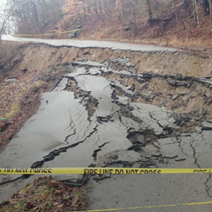
The Mud Creek landslide near Big Sur, California, dumped about 6 million cubic yards (5 million cubic meters) of rock and debris across California Highway 1 on May 20, 2017.
The Mud Creek landslide near Big Sur, California, dumped about 6 million cubic yards (5 million cubic meters) of rock and debris across California Highway 1 on May 20, 2017. Credit: U.S. Geological Survey

Landslides are some of the most common disasters in the world, killing thousands of people each year. The mass movement of land (sediments and soils, bedrock and boulders, even whole mountainsides) down a slope is induced by the force of gravity. There are numerous contributing forces to a landslide, many of which can be monitored or observed through remote sensing data. Intense or prolonged rainfall is the most frequent extrinsic trigger of landslides, as it reduces friction between materials and increases the water pressure within the soil pores, increasing the likelihood of failure. Earthquakes and changes to the landscape from wildfires, road building, and deforestation can also contribute to the instability of the land surface and cause landslides. NASA's Earth observation data provide important data to estimate landslide hazards. Within the U.S., the United States Geological Survey's (USGS) National Landslide Hazards Program provides important information on identifying and monitoring landslides.

Please visit the Earthdata Forum, where you can interact with other users and NASA subject matter experts on a variety of Earth science research and applications topics.

Find the Data

event-monitoring
Knowing where and when landslides occur can help communities worldwide prepare. NASA datasets, like precipitation, soil moisture, freeze/thaw conditions allow for modeling and forecasting, which can help researchers understand areas of potential concern.
post-event-impacts
Every year landslides block roads, damage infrastructure, and cause thousands of fatalities. NASA datasets provide means of measuring ground deformation, landslide extent, and community vulnerabilities.
Tools for Data Access and Visualization

Earthdata Search | Panoply | Giovanni | Worldview | AppEEARS | Soil Moisture Visualizer | MODIS/VIIRS Subsetting Tools Suite | Sentinel Toolbox

Earthdata Search

Earthdata Search is a tool for data discovery of Earth Observation data collections from NASA's Earth Observing System Data and Information System (EOSDIS), as well as U.S and international agencies across the Earth science disciplines. Users (including those without specific knowledge of the data) can search for and read about data collections, search for data files by date and spatial area, preview browse images, and download or submit requests for data files, with customization for select data collections.


Screenshot of the Search Earthdata site.

In the project area, for some datasets, you can customize your granule. You can reformat the data and output as HDF, NetCDF, ASCII, KML, or a GeoTIFF. You can also choose from a variety of projection options. Lastly, you can subset the data, obtaining only the bands that are needed.


Earthdata Search customization tools diagram.

Panoply

HDF and NetCDF files can be viewed in Panoply, a cross-platform application that plots geo-referenced and other arrays. Panoply offers additional functionality, such as slicing and plotting arrays, combining arrays, and exporting plots and animations.

Giovanni

Giovanni is an online environment for the display and analysis of geophysical parameters. There are many options for analysis. The following are the more popular ones.

  • Time-averaged maps are a simple way to observe the variability of data values over a region of interest.
  • Map animations are a means to observe spatial patterns and detect unusual events over time.
  • Area-averaged time series are used to display the value of a data variable that has been averaged from all the data values acquired for a selected region for each time step.
  • Histogram plots are used to display the distribution of values of a data variable in a selected region and time interval.

For more detailed tutorials:

  • Giovanni How-To’s on NASA's Goddard Earth Sciences Data and Information Services Center (GES DISC) YouTube channel.
  • Data recipe for downloading a Giovanni map as NetCDF and converting its data to quantifiable map data in the form of latitude-longitude-data value ASCII text.

Worldview

NASA's EOSDIS Worldview visualization application provides the capability to interactively browse over 1,000 global, full-resolution satellite imagery layers and then download the underlying data. Many of the available imagery layers are updated within three hours of observation, essentially showing the entire Earth as it looks "right now." This supports time-critical application areas such as wildfire management, air quality measurements, and flood monitoring. Imagery in Worldview is provided by NASA's Global Imagery Browse Services (GIBS). Worldview now includes nine geostationary imagery layers from Geostationary Operational Environmental Satellite (GOES)-East, GOES-West and Himawari-8 available at ten minute increments for the last 30 days. These layers include Red Visible, which can be used for analyzing daytime clouds, fog, insolation, and winds; Clean Infrared, which provides cloud top temperature and information about precipitation; and Air Mass RGB, which enables the visualization of the differentiation between air mass types (e.g., dry air, moist air, etc.). These full disk hemispheric views allow for almost real-time viewing of changes occurring around most of the world.


Image
Worldview data visualization of the nighttime lights in Puerto Rico pre- and post- Hurricane Maria, which made landfall on September 20, 2017. Post-hurricane image shows widespread outages around San Juan, including key hospital and transportation infrastructure.
Worldview Suomi NPP/VIIRS nighttime lights comparison image showing power outages caused by Hurricane Irma in September 2017. The right image (acquired 1 September 2017) shows the island before Hurricane Irma. The left image (acquired 9 September 2017) shows power outages across island after Hurricane Irma. NASA Worldview image.

AppEEARS

AppEEARS, from LP DAAC, offers a simple and efficient way to access and transform geospatial data from a variety of federal data archives. AppEEARS enables users to subset geospatial datasets using spatial, temporal, and band/layer parameters. Two types of sample requests are available: point samples for geographic coordinates and area samples for spatial areas via vector polygons.

Performing Area Extractions

After choosing to request an area extraction, you will be taken to the Extract Area Sample page where you will specify a series of parameters that are used to extract data for your area(s) of interest.

Spatial Subsetting

Define your region of interest in one of these three ways:

  • Upload a vector polygon file in shapefile format (you can upload a single file with multiple features or multipart single features). The .shp, .shx, .dbf, or .prj files must be zipped into a file folder to upload.
  • Upload a vector polygon file in GeoJSON format (can upload a single file with multiple features or multipart single features).
  • Draw a polygon on the map by clicking on the Bounding box or Polygon icons (single feature only).

Select the date range for your time period of interest.

Specify the range of dates for which you wish to extract data by entering a start and end date (MM-DD-YYYY) or by clicking on the Calendar icon and selecting dates a start and end date in the calendar.

Adding Data Layers

Enter the product short name (e.g., MOD09A1, ECO3ETPTJPL), keywords from the product long name, a spatial resolution, a temporal extent, or a temporal resolution into the search bar. A list of available products matching your query will be generated. Select the layer(s) of interest to add to the Selected layers list. Layers from multiple products can be added to a single request. Be sure to read the list of available products available through AppEEARS.


Extracting an area in AppEEARS
Selecting Output Options

Two output file formats are available:

  • GeoTIFF
  • NetCDF-4

If GeoTIFF is selected, one GeoTIFF will be created for each feature in the input vector polygon file for each layer by observation. If NetCDF-4 is selected, outputs will be grouped into .nc files by product and by feature.


If GeoTIFF is selected, you must select a projection
Interacting with Results

Once your request is completed, from the Explore Requests page, click the View icon in order to view and interact with your results. This will take you to the View Area Sample page.

The Layer Stats plot provides time series boxplots for all of the sample data for a given feature, data layer, and observation. Each input feature is renamed with a unique AppEEARS ID (AID). If your feature contains attribute table information, you can view the feature attribute table data by clicking on the Information icon to the right of the Feature dropdown. To view statistics from different features or layers, select a different AID from the Feature dropdown and/or a different layer of interest from the Layer dropdown.


Interpreting Results in AppEEARS

Be sure to check out the AppEEARS documentation to learn more about downloading the output GeoTIFF or NetCDF-4 files.

Soil Moisture Visualizer

ORNL DAAC has developed a Soil Moisture Visualizer tool (read about it at Soil Moisture Data Sets Become Fertile Ground for Applications) that integrates a variety of different soil moisture datasets over North America. The visualization tool incorporates in-situ, airborne, and remote sensing data into one easy-to-use platform. This integration helps to validate and calibrate the data, and provides spatial and temporal data continuity. It also facilitates exploratory analysis and data discovery for different groups of users. The Soil Moisture Visualizer offers the capability to geographically subset and download time series data in .csv format. For more information on the available datasets and use of the visualizer, view the Soil Moisture Visualizer Guide.

To use the visualizer, select a dataset of interest under Data. Depending on the dataset chosen, the visualizer provides the included latitude/longitude or an actual site location name and relative time frames of data collection. Upon selection of the parameter, the tool displays a time series with available datasets. All measurements are volumetric soil moisture. Surface soil moisture is the daily average of measurements at 0-5 cm depth, and root zone soil moisture (RZSM) is the daily average of measurements at 0-100 cm depth. Lastly it provides data sources for download.


Image
ORNL DAAC Soil Moisture Visualizer
The Soil Moisture Visualizer allows users to compare soil moisture measurements from multiple sources (figure legends, top left and bottom right) at the same location. In this screenshot, Level 4 Root Zone Soil Moisture (L4 RZSM) data from NASA’s Soil Moisture Active Passive (SMAP) Observatory are shown with data from in situ sensors across the 9-kilometer Equal-Area Scalable Earth (EASE) grid cell encompassing the Tonzi Ranch Fluxnet site in the Sierra Nevada foothills of California. Daily precipitation values for the site (purple spikes) are also provided for reference.

MODIS/VIIRS Subsetting Tools Suite

ORNL DAAC also has several MODIS and VIIRS Subset Tools for subsetting data.

  • With the Global Subset Tool, you can request a subset for any location on earth, provided as GeoTIFF and in text format, including interactive time-series plots and more. Users specify a site by entering the site's geographic coordinates and the area surrounding that site, from one pixel up to 201 x 201 km. From the available datasets, you can specify a date and then select from MODIS Sinusoidal Projection or Geographic Lat/Long. You will need an Earthdata Login to request data.
  • With the Fixed Subsets Tool, you can download pre-processed subsets for 3000+ field and flux tower sites for validation of models and remote sensing products. The goal of the Fixed Sites Subsets Tool is to prepare summaries of selected data products for the community to characterize field sites. It includes sites from networks such as NEON, ForestGeo, PhenoCam and LTER that are of relevance to the biodiversity community.
  • With the Web Service, you can retrieve subset data (in real-time) for any location(s), time period, and area programmatically using a REST web service. Web service client and libraries are available in multiple programming languages, allowing integration of subsets into users' workflow.


Image
Directions for subsetting data with the ORNL DAAC MODIS and VIIRS subset tool
Top image: The Global Subsets Tool enables users to download available products for any location on Earth. Bottom image: The Fixed Sites Subsets Tool provides spatial subsets for established field sites for site characterization and validation of models and remote sensing products.

Sentinel Toolbox

The European Space Agency (ESA) Sentinel-1 Mission consists of two satellites, Sentinel-1A and Sentinel-1B, with SAR instruments operating at a C-Band frequency. They orbit 180° apart, together imaging the entire Earth every six days. SAR is an active sensor that can penetrate cloud cover and vegetation canopy, and also observe at night. It also provides useful information to detect movement of Earth material after an earthquake, volcanic eruption or landslide. SAR data are very complex to process, however, ESA has developed a Sentinel-1 Toolbox to aid with processing and analysis of Sentinel-1 data.

For more information on active sensors, see What is Remote Sensing.

SAR Interferometry

Once you have downloaded the data, a data file before the event and a data file after the event, you will need to coregister the two files and then create an interferogram. The process for doing that follows:

  1. Visualize: Open the files in the Sentinel Toolbox. Important note: DO NOT unzip the downloaded SAR file. When you expand the Bands folder, you will find bands containing the real (i) and imaginary (q) parts of the complex data. In Sentinel-1 IW SLC products, you will find three sub-swaths labeled IW1, IW2, and IW3. To view the data, double-click on the Intensity Sub-Swath Polarization band of one of the two images.
  2. Coregister: For interferometric processing, two or more images must be coregistered into a stack. One image is selected as the master and the other images are the "slaves." The pixels in "slave" images will be moved to align with the master image to sub-pixel accuracy. To do this, select Radar/Coregistration/S-1 TOPS Coregistration. For more information on this type of processing, view Sentinel Online's Terrain Observation with Progressive Scans SAR (TOPSAR) processing technique.
    1. In the Read tab, select the first product. This should be the earlier of the two SLCs.
    2. In the Read(2) tab, select the other product. This will be your "slave" image.
    3. In the TOPSAR-Split tabs, select the appropriate sub-swath and polarization for each of the products.
    4. In the Apply-Orbit-File tabs, select the Sentinel Precise Orbit State Vectors. If precise orbits are not yet available for your product, you may select the restituted orbits, which may not be as accurate but will be better than the predicted orbits available within the product.
    5. Image
      Sentinel-1 Toolbox coregistration process. Note the arrow to the left and right in the coregistration window; it will cycle through the different tabs.
      Sentinel-1 Toolbox coregistration process. Note the arrow to the left and right in the coregistration window; it will cycle through the different tabs.
      In the Back-Geocoding tab, select the DEM to use and the interpolation methods. The default is the SRTM 3 Sec DEM.
    6. In the Write tab, set the Directory path to your working directory.
    7. Click Run to begin coregistering the data. The resulting coregistered stack product will appear in the Product Explorer window with the suffix Orb Stack.
  3. Interferogram: The interferogram is formed by cross-multiplying the master image with the complex conjugate of the "slave." The amplitude of both images is multiplied while their respective phases are differenced to form the interferogram.
    1. Select the new stack file in the product explorer and then select Radar/Interferometric/Products/Interferogram Formation.
    2. Keep the default values for Interferogram Formation, but confirm that the output Directory path is correct.
    3. Click Run.
    Image
    Sentinel-1 Toolbox interferogram
    Through the interferometric processing flow, the tool tries to eliminate other sources of error so that what is left is typically the surface deformation related to an event. You can visualize the phase information at this step.

    Interferometric fringes represent a full 2π cycle of phase change. Fringes appear on an interferogram as cycles of colors, with each cycle representing relative range difference of half a sensor's wavelength. Relative ground movement between two points can be calculated by counting the fringes and multiplying by half of the wavelength. The closer the fringes are together, the greater the strain on the ground.

  4. Multilooking and Phase Filtering: Lastly the phase associated with topography has to be removed and additional phase filtering to reduce noise and enhance the appearance of the deformation fringes.

Step-by-steps of this can be found within ASF DAAC's InSAR data recipes.

Last Updated