Description

The Hurricane and Severe Storm Sentinel (HS3) airborne field campaign used the Cloud Precipitation Lidar (CPL) instrument to collect measurements of cloud, precipitation, and aerosol features of tropical cyclones. This data recipe instructs users on how to generate vertical time-height plots of HS3 CPL attenuated total backscatter measurements using a Python plotting routine. The Python routine requires users to define the GHRC OPeNDAP path to a datafile and the spectral channel the measurements were collected. To run this Python routine, a pre-installed version of Python and additional Python packages are required. Advanced users may alter the code to plot other data variables. 
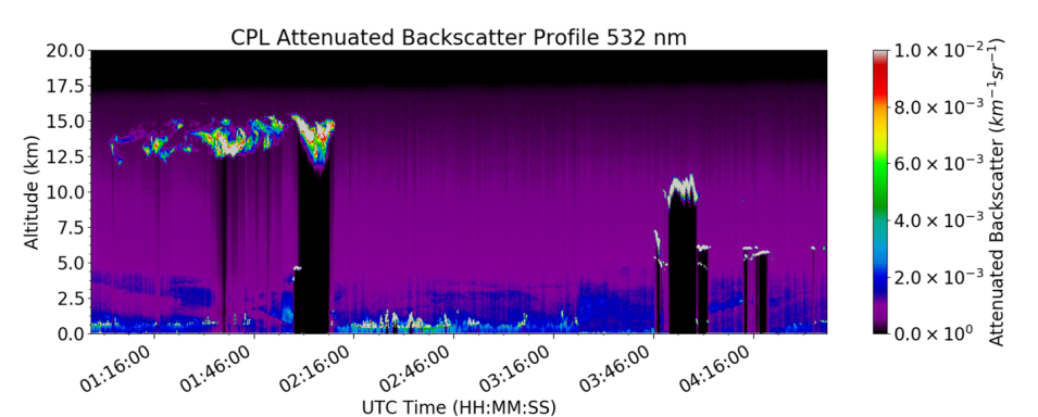
Time-height plot of HS3 CPL 532 nm attenuated total backscatter collected on September 6, 2012
Image Caption

Time-height plot of HS3 CPL 532 nm attenuated total backscatter collected on September 6, 2012

Supporting Software Information

TypeAccess
iPython NotebookOpen Source
Python ScriptLocation

How to use

This data recipe uses the Hurricane and Severe Storm Sentinel (HS3) Global Hawk Cloud Physics Lidar (CPL) HDF-EOS5 dataset. More information and additional resources about this dataset can be accessed here.
 
In addition, this data recipe is available as a Python script and an iPython Notebook, which is an interactive Python environment for the web and shell. To run the Python script and iPython Notebook, please install the following Python modules: matplotlib, NumPy, Pydap, SciPy, and mpmath
 

Step 1

Follow the location link on this page to access the GHRC DAAC data-recipe GitHub folder. The HS3 CPL Attenuated Total Backscatter Quick View has two separate files available for download: an iPython Notebook and Python Script.
 
You can preview each by clicking the file name. To download, select the green “Clone or download” button located on the right side of the webpage to download both scripts as a zipped file or to open them on your desktop. Save both or either files to the desired folder location on your computer.

Step 2

Open the Python environment installed on your computer and make sure the required Python packages outlined in the “How to Use” section are installed. 
 
Navigate to the location on your computer where the data recipe Python file is saved and open the file within your Python environment.

Step 3

The Python script provides a series of editable fields used to plot desired parameters and locations recorded within each HS3 CPL data file. This data recipe uses OPeNDAP to access the data so that users do not need to download and save data files to their computers.  
 
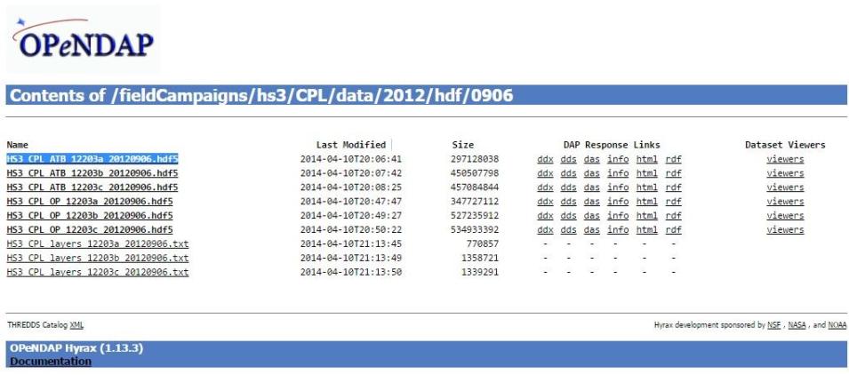
To define the datafile you want to use, navigate to the GHRC HS3 CPL OPeNDAP directory.  The HS3 CPL datafiles are organized by year.  Select 2012 to plot the figure in this example.
Screenshot of the OPeNDAP data directory.

Then select the link for “hdf/” as shown below.

Screenshot of the OPeNDAP data directory

The next directory contains files organized by date in YYYYMMDD format. Select your date of interest, or September 6th, 2012 to generate the example plot created for this data recipe. Copy the desired file name as shown.

Screenshot of the OPeNDAP data directory

Step 4

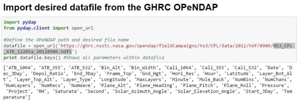
Within the Python script, to change the default data file to one you want to use, simply paste your file name to the "datafile" variable in the region highlighted below. Make sure to update the OPeNDAP URL path to reflect the year and day of the datefile.

Screenshot of code block for data file.

Step 5

This data recipe plots the CPL attenuated total backscatter (ATB) for 532 nm, 1064 nm, and 355 nm. For the example plot shown, the 532 nm data are used to create the plot.  
 
To change the desired channel, simply change the variable “var_ATB” in the code within the highlighted section below to “ATB_1064” to plot the 1064 nm channel, or “ATB_355” to plot the 355 nm channel.
Screenshot of code block with parameters highlighted.

Step 6

The proceeding code extracts and formats the necessary parameters within the HDF-EOS5 datafile to create a vertical time-height plot of the HS3 CPL data.
 
The final section of the code formats the plot. You may alter the code to tailor the color scale, text size, text content, and plot parameters to your liking. Note that the current title of the generated plot states the 532 nm channel was used. When creating a plot of another channel remember to change the highlighted title text below.
Screenshot of code block with parameters highlighted.

Step 7

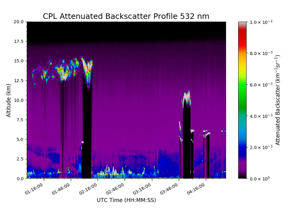
To create the data plot, simply run the script. A window will pop up containing the desired plot.

CPL Attenuated Backscatter
Image Caption

This data requires additional processing to quality control and remove erroneous data values.  Please refer to the User Guide and PI Documentation for additional information on data quality. 

Step 8

If you would like the run this data recipe as an iPython Notebook, run externally through the Jupyter Notebook web application. More information on Jupyter can be found on the Jupyter site.

The Python script and iPython Notebook may be reused and altered to plot additional CPL data variables not used in this data recipe. Additional documentation is provided within the code to help walk you through the content.

Dataset Information

Dataset NameHurricane and Severe Storm Sentinel (HS3) Global Hawk Cloud Physics Lidar (CPL)
PlatformGlobal Hawk Unmanned Aerial Vehicle (UAV)
InstrumentCloud Precipitation Lidar (CPL)
Science ParameterAttenuated Total Backscatter
FormatHDF-EOS5
Data InformationCMR Search

Key Parameters

VariableDescriptionDimensionUnitsScale Factor
timeTimen/asecondsnone
bin_AltAltitude in km for each vertical bin1Dkilometernone
Dec_JDayDecimal day of year to 5 decimal places (second) for current profile1Ddays since 2012-01-01T00:00:00Znone
DateDate for flight1Dtextnone
ATB_1064Attenuated total backscatter collected for 1064 nm channel2Dkm-1 sr-1none
ATB_355Attenuated total backscatter collected for 355 nm channel2Dkm-1 sr-1none
ATB_532Attenuated total backscatter collected for 532 nm channel2Dkm-1 sr-1none

Details

Last Updated

Published on

Data Centers

Global Hydrometeorology Resource Center DAAC (GHRC DAAC)