On a hilly peninsula overlooking the Pacific Ocean and San Francisco Bay, 5,000 miles of pipeline zigzag over Richmond, California. The Chevron Richmond Refinery, established in 1902, is one of five refineries in the East Bay region, coined “refinery corridor,” where industrial grids dominate and stacks disrupt the horizon. Air quality has been an issue here for over a century, but recently the invisible ingredients—the health-damaging pollutants and warming greenhouse gases—are of major concern in the backdrop of climate change.
California’s 2016 bill is intended to give lawmakers more oversight of the state’s Air Resources Board with a goal of reducing 40 percent of greenhouse gas emissions by 2030 and 80 percent by 2050. As Nick Parazoo, a researcher at NASA's Jet Propulsion Laboratory put it, “There is no easy way of verifying whether that is going to happen or not.” To help lawmakers know if targets have been met, a group of scientists led by Heather Graven at Imperial College in London created a simulation, or a theoretical case study, to see how best to increase confidence in greenhouse gas emission measurements.

The measure of life and death
Typical measurements of fossil fuel emissions look at fuel consumption, and the potential carbon dioxide (CO2) within that fuel. On a global scale, accuracy can be within 5 percent, but testing fossil fuel emission on a regional scale requires isolating factors that easily cross arbitrary borders, such as wind blowing across California state lines.
By modeling the motion of air over California in fine detail, the researchers could observe where air came from, how it moved, and how it interacted with the environment. “We’re basically looking at the difference between what’s in California and what’s flowing into California as a way of judging what California must have added or subtracted,” said Marc Fischer, an atmospheric scientist at Lawrence Berkeley National Laboratory.
Only four hundredths of a percent of air is composed of CO2, a heat-trapping greenhouse gas. Methane (CH4) warrants equal attention as an emission source from cows, landfills, and gas leaks, but limitations in satellite instrumentation, which have yet to detect methane, led the researchers to focus solely on CO2 emissions.
All life respires, releasing CO2 into the atmosphere, but plants do more. “Plants are supremely beautiful living organisms because they are both breathing in CO2 during the day and breathing it out at night,” Fischer said. During photosynthesis, plants absorb CO2 and sunlight to create fuel—glucose and other sugars—to build plant structures. This accumulation of CO2 as biomass in plants removes CO2 from the atmosphere.
Measuring CO2 in the biosphere, where exchanges occur between living organisms, gets complicated because life is dynamic. Seasons shift, droughts happen, and plant metabolism decreases. To differentiate between fossil fuel emissions, which also spew CO2 into the atmosphere, the team traced the origins of the carbon molecules. All life, living and long dead as with fossil fuels, is composed of carbon. Carbon holds six protons, but can have a different number of neutrons in its nuclei, thus changing its mass to become an isotope. Carbon has two stable isotopes, 12C and 13C, and the unstable, radioactive 14C, also called radiocarbon, with a half-life of 5,700 years.
When solar particles smack into the upper atmosphere, they form a tiny, continuous amount of 14C, which plants incorporate through photosynthesis and animals by eating plants. When an animal dies, carbon is no longer exchanged with its environment, and radiocarbon begins to decay. The older a sample, the less radiocarbon it carries. Fossil fuels, or decayed organic matter that has been underground for millions of years, contain no radiocarbon. So a big drop of radiocarbon in the atmosphere indicates a rise in fossil fuel emissions.

A tower for all seasons
Measuring radiocarbon accurately can be tricky because the atmosphere contains little radiocarbon. For every 14C atom there are a trillion 12C atoms. Faint CO2 clouds swirl in the atmosphere, and the most accurate method to measure them requires capturing air in a flask, and then taking it to a lab. “It’s the most precise measurement you can get, but it’s also expensive,” Parazoo said. Hence, the study also considered data from a tower network and data that simulates the NASA Orbiting Carbon Observatory-2 (OCO-2) satellite. Since OCO-2 launched in July 2014 and the first observations were under scientific analysis, no actual data were used for this simulation. Instead, synthetic results were generated using the OCO simulator at Colorado State University.
In addition to being the sites of flask sampling, the 10 towers could continuously measure the carbon exchange, providing total CO2 calculations, which offered an in-depth look at the biosphere exchange through the seasons. “What we’re doing is not completely new,” Fischer said, “but it will be the first time researchers have used OCO-2 data in combination with radiocarbon data to tell the bigger story of fossil fuels and the biosphere.” For this study, however, only the flask samples were used, though the researchers note that the addition of continuous CO2 data could improve estimates of CO2 exchange in future studies.
The towers measured close to the surface, about two meters high. Ninety-five percent of air particles hover at that level, but gases in the atmosphere mix at different heights depending on the weather. Things shift up on hot, dry days and down on cooler days. “The thing about OCO-2 is it looks through the entire column, from space to surface, and estimates the average concentration for the entire column,” Fischer said. That has an advantage over the tower measurement.
Large-scale patterns of CO2 on a global scale are expected: Earth’s Northern Hemisphere greens in the summer, breathing in CO2, and browns in winter while breathing out CO2. OCO-2 detects those oscillations, but Parazoo was skeptical the satellite would detect useful information from thousands of miles away. The challenge is that a CO2 particle is hard to track because OCO-2 has a long observation cycle. Once emitted, CO2 moves through life close to the surface, but once it gets carried away from the surfaces and mixes with the background atmosphere, it gets smoothed out. By the time OCO-2 returns 16 days later, the CO2 particle is long gone.
In addition, a column can have a value of 400 parts per million (ppm), but to understand something about climate change the precision must be crazy sensitive to detect changes, which occur at about 2 ppm.
The biosphere element is key to determine yearly emission levels because years of drought remove less CO2 than non-stressed years. “With climate change, and warming and drying, you are affecting the ability of plants to grow in response to increasing carbon,” Parazoo said. To isolate fossil fuel combustion, the team had to estimate the total carbon exchange, a mixture of biosphere and fossil fuel emission. Then, the fossil fuel portion could be subtracted, leaving only the biosphere contribution on a daily, seasonal, inter-seasonal, and year-to-year scale.

Simulation sandwich
The results are part of a hypothetical scenario, using CO2 exchange data for May 2011 and November 2010, dates that were simply a matter of convenience. In May, the biosphere is wide awake, increasing the sink of CO2. In November, the biosphere sleeps and the dominating carbon signal comes from fossil fuel emissions.
The simulation creates an alternate reality where researchers can predict CO2 concentrations based on a fossil fuel emission scenario. Then they become architects, designing a system that reflects a given quantity. “The simulation is more of a thought experiment to see if it’s possible to get the desired result of an emission measurement,” Parazoo said. Specifically, this simulated world took different estimates of fossil fuel emissions, averaged them, and then created synthetic observations to detect simulated changes in the fossil fuel emissions. “What you want is to verify that your experimental setup works so you can apply it to real observations, and understand the results,” Parazoo said. “The uncertainty reduction tells you it works.”
The simulation is a competition between initial emission sources and the addition of observed sources. More observation can identify flaws in prior knowledge and reduce uncertainty. “In a perfect world, you would have an unlimited amount of observations over California. Then your uncertainty theoretically would go down to zero,” Parazoo said.
The combination of flask measurements and satellite observation dropped uncertainty to 5 to 10 percent over California. “I am surprised about how much work it is to get this problem of emissions,” Fisher said. “It is not easy.” Right now, California is on track to meet its 2020 deadline: cutting greenhouse gas emission by 15 percent. The next step is to run the model with actual, instead of simulated satellite measurements to help officials target California’s biggest polluters and to help communities breathe easier.

References
Fischer, M. L., N. C. Parazoo, K. Brophy, X. Cui, S. Jeong, J. Liu, R. Keeling, T. E. Taylor, K. R. Gurney, T. Oda, and H. Graven. 2017. CMS: CO2 Signals Estimated for Fossil Fuel Emissions and Biosphere Flux, California. ORNL DAAC, Oak Ridge, TN, USA. doi:10.3334/ORNLDAAC/1381.
Fischer, M. L., N. Parazoo, K. Brophy, X. Cui, S. Jeong, J. Liu, R. Keeling, T. E. Taylor, K. Gurney, T. Oda, and H. Graven. 2017. Simulating estimation of California fossil fuel and biosphere carbon dioxide exchanges combining in situ tower and satellite column observations. Journal Geophysical Research: Atmospheres 122: 3,653–3,671. doi:10.1002/2016JD025617.
O’Brien, D. M., I. Polonsky, C. O’Dell, and A. Carheden. 2009. Orbiting Carbon Observatory (OCO) Algorithm Theoretical Basis Document: The OCO Simulator. Cooperative Institute for Research in the Atmosphere: Colorado State University, Fort Collins.
OCO-2 Science Team/Michael Gunson, Annmarie Eldering. 2015. OCO-2 Level 2 geolocated XCO2 retrieval results and algorithm diagnostic information V7, Greenbelt, MD, USA, Goddard Earth Sciences Data and Information Services Center (GES DISC), https://disc.gsfc.nasa.gov/datacollection/OCO2_L2_Diagnostic_7.html.
For more information
NASA Goddard Earth Sciences Data and Information Services Center (GES DISC)
NASA Oak Ridge National Laboratory Distributed Active Archive Center (ORNL DAAC)
NASA Orbiting Carbon Observatory-2 (OCO-2)
| About the data | ||
|---|---|---|
| Satellite | Orbiting Carbon Observatory (OCO-2) | |
| Project | Carbon Monitoring System (CMS) | |
| Data sets | OCO-2 Level 2 Geolocated XCO2 Retrieval Results and Algorithm Diagnostic Information V7 | CMS: CO2 Signals Estimated for Fossil Fuel Emissions and Biosphere Flux, California |
| Temporal resolution | 16 days | November 1, 2010 to May 31, 2011 |
| Resolution | 2.25 x 1.29 kilometer | |
| Parameter | Carbon dioxide | Carbon dioxide |
| DAACs | NASA Goddard Earth Sciences Data and Information Services Center (GES DISC) | NASA Oak Ridge National Laboratory Distributed Active Archive Center (ORNL DAAC) |
| The study used simulated data generated with the OCO simulator at Colorado State University. | ||